A simpler way to reduce laser rangefinder data

The raw data

The SICK LMS laser rangefinder gives us a line scan of 361 range data points spread over 180 degrees. There are 75 scans per second. This works out to about one point per 20 cm in each axis at maximum range and speed. That's our starting point. We also have INS/GPS information about vehicle speed, roll, and pitch.

Line scan data

We want to measure local terrain tilt and roughness, for which we need the data for a point and its neighbors in some consistent coordinate system. "Tilt" is obtained by fitting a plane to a small number of nearby points. "Roughness" is the standard deviation from that plane. These give us enough data to determine whether a piece of terrain can be traversed.

We first translate each data point into a 2D point in the plane of the scan, with the origin at the rangefinder. This is just a conversion from radial to Cartesian coordinates. The cheapest way to do this is to pre-compute the unit vectors for the 361 directions the laser rangefinder can scan, and multiply each measured point by the appropriate unit vector. The special values the LMS produces (no return, blinded by glare) must also be handled.

The processing is very localized. Rather than trying to build a point cloud, we only need to work on three scan lines at a time. On each line scan cycle, we must look at each point in the middle scan line, its neighbors in the current scan, and its nearest neighbors in the adjacent scan lines. We need to look up to 9 points total per set.

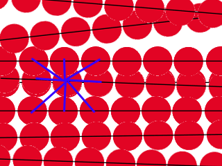
Line Scan Pattern This is a top view of the pattern scanned by the laser rangefinder. Each red dot represents one measured value, and each row of red dots is one scan line. Each scan line can be assumed to be straight, but the alignment from scan line to scan line can vary considerably, since it is determined by vehicle movement. Roll results in a tilt of the scan line. Pitch varies the distance between the scan lines. For each point, we must find the neighboring points. We need only look at three scan lines at a time, which simplifies processing. Each point has up to eight neighbors, two on the current scan line and up to three on each adjacent scan line, as illustrated in blue.

The minimal information we need to do this processing for a set of three scan lines is the LMS data, forward speed, roll rate, pitch rate, and scanner tilt angle. We can get the needed relative pitch and roll angles between scan lines by integrating roll rate and pitch rate over one scan line time. This gives us tilt vectors and roughness data in the coordinate system of the middle scan line being worked on.

The line scan data can be processed linearly, progressing across the middle line of the three stored lines. The neighbors on the current line are just the previous and next points. The neighbors on the adjacent lines are a bit tougher to determine, because the lines may be offset in both pitch and roll. But it's not that hard.

The output of this stage is a row of tilt vectors and roughness data in the coordinate system of the middle scan line. We get one such data item every scan line time.

Local drivability

Here's an initial set of rules.

• Any point with more than 20 cm of roughness is not driveable
• Any point with more than 15 degrees of tilt (any axis) is not driveable
• Any point with less than five measured neighbors is not driveable

This is probably too conservative. But it's a good starting point.

Transforming the data into a map

Transforming the data points into a consistent coordinate system is the inverse of the process by which graphics programs map data points from a 3D model on a 2D screen, and can be performed by one 4x4 matrix multiply.

What we need is a 4x4 transformation matrix which transforms these 2D points into 3D points in a consistent coordinate system
("world space"). The information for this matrix comes from the GPS/INS server, and the encoder for the laser rangefinder tilt head.

The output coordinate system is that of the current local map.

Vector field output

One output of this process is a 3D vector field, with normal vectors for each scanned point, a "roughness" value for each scanned point, and a "confidence" value, representing how many good data points went into this datum. ("Confidence" here is probably best reduced to a Boolean value; if we have at least five good points contributing to a normal vector, it's a good point.).

A simplified system

Here's a somewhat simpler approach.

Simplified line scanning

First, line scan data is interpreted, as above, working on three scan lines at a time. But we assume that the vehicle does not move much between the two scan lines. Our scan rate is 75 Hz If we can damp the movement of the scanner base enough that there's little vibration above 25 Hz, we can perform the three-line comparison very simply, without applying corrections for every point. All we have to do is take the vehicle's up vector (from the INS) and use it to align the up vectors from the laser rangefinder with the real world. On flat terrain, we don't even have to do that.

On near-flat terrain, this is enough. On rougher terrain, there are problems.

Simplified mapping

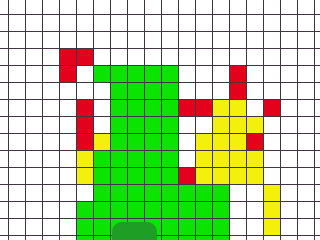
The world is divided into squares colored red, green, yellow, and blank.

Near-area map RED (3) - not driveable YELLOW (2) - data available, more analysis required GREEN (1) - driveable BLANK (0) - no data available

From the line scanning above, we can initially classify squares. Green squares are flat - low roughness (< 5-10 cm variation) and low tilt (< 10 degrees). Red squares are high roughness or tilt. Yellow squares are in between.

Yellow squares require more processing because we may have to consider them in conjunction with adjacent squares to decide whether they're driveable. Green squares are so flat and level that we can treat any green area as passable, and don't have to evaluate those areas in more detail.

As a first cut, we can treat yellow squares as impassable, or red. Unless we don't have a path available over green squares only, we don't need to evaluate yellow squares further.

Positive (above the ground) obstacles will be seen on successive scans but at different heights. Each three-line group which includes a positive obstacle should result in a red square. We never want to ignore a positive obstacle. Hence, during updating, red should supersede yellow, yellow should supersede green, and green should supersede blank. Or, higher numbers replace lower numbers.

Negative (below the ground) obstacles often won't be seen at all from a distance, because they are occluded by the terrain in front of them. They thus show as blank areas in the map.

The output of all this feeds into the field-based OpenSteer system, of course.

Processing of ambiguous (yellow) areas.

Yellow areas may or may not be driveable by our vehicle. For yellow areas, we need to do a more complex evaluation. We need to evaluate patches the size of our vehicle, and decide whether we can drive over that area.

***MORE***

This should be a lazy-evaluation system, where we don't evaluate a yellow square unless the field based system needs information about it.

To do:

- How do multiple scans update a square? Do we need absolute height?

-- For red and yellow squares, absolute height is important, so we can recognize big height changes. It's not too important for green squares, because they're so flat. Absolute height is noisy, so we don't want to use it too much.

- Multiple data points into the same square on multiple scans can turn a square red if there's a big height variation. Do we need to do more than the three-line comparison?

- A later scan can turn a square red.

- What happens when we see a fence?

- Active control of the laser rangefinder to fill in holes in the data.